Blob Family

Physically-based simulation is becoming increasingly important in both animation and game production, the use of physically-based gameplay provides a wonderful means for players to immerse themselves within a game, and games such as Gish and LocoRoco base their entire gameplay around a 2D blob (Gish's source code has been open sourced, for those brave enough to dive in).

Articles on blob simulation is surprisingly sparse on the Web, looking over related papers and discussions on soft body dynamics, a mass-spring system utilizing Verlet integration and constraints is the most popular choice. A successful (and happy) blob implemented with a mass-spring system requires a combination of several complimentary techniques:

• Mass-spring system modeling point mass as particles with semi-rigid constraints
• Use Verlet integration to update particle position based on accumulated forces
• A simple collision handling engine
• Rendering engine that can turn the point masses into a blobby object

Blob Family simulates a group of blobs generated through physical simulation. The program is created in Processing, but the code can easily be ported to JavaScript. A downloadable version of the simulation is available at the bottom of this page.

# Mass Spring System

If you think about it, a blob is really just a type of very viscous fluid, so one may try to implement some kind of fluid simulation with constraints. However, fluid simulation can be quite difficult to get right and is computationally demanding, all we really want is the appearance of a fluid-looking, deformable object. Under most circumstances, a simpler (and sometimes less realistic) system can be used as long as it creates believable simulation.

In a mass-spring system, we model the blob as a system of point masses (particles) connected by a series of springs in the shape of a blob.

A point mass is an object with properties such as mass, position, and force. During simulation, the program iterates through each particle, accumulates all forces currently acting on the particle, applies the total force to that particle's position using Verlet integration, and finally computes constraints to stabilize the overall system.

During the force accumulating stage, all forces currently acting on the particle are added up, including environmental forces like gravity, player stimulated movements, and last but not least, spring forces from neighboring particles. Since particles in our system are connected to each other through springs, the springs will compress and stretch, causing the entire system to wobble around like a blob would. Depending on the spring's elasticity, the blob can be made to appear bouncy or slippery, or even as a rigid body.

Since the particles are connected by spring, the connections obey Hooke's law of elasticity:

F = k * Δx

Where Δx is the distance between spring length and rest length, and k is the spring elasticity (stiffness). For x < x_rest, the spring wants to extend, for x > x_rest, the spring wants to contract.

According to Hooke's law, the force needed to extend or compress a spring back to its rest length is the distance between its current length and its rest length, multiplied by spring elasticity.

Putting it all together, we arrive at the force accumulation code.

// For each particle
force.set(0.0, 0.0); // Reset force

// Apply gravity if enabled
if (enable_gravity) force += gravity * mass;

// Keyboard input
if (keys[UP]) force += Vector(0.0, -60.0);
if (keys[LEFT]) force += Vector(-60.0, 0.0);
if (keys[DOWN]) force += Vector(0.0, 60.0);
if (keys[RIGHT]) force += Vector(60.0, 0.0);

// Gather forces from all connected constraints for all particles
for (int i = 0; i < num_of_links; j++) {
    // Obeys Hook's law: f = k * (x - x0)
    // Vector from neighbor to self
    Vector it2me = pos - neighbor_pos;
    // Vector from neighbor to rest position, MID is length of spring at rest
    Vector it2mid = neighbor_pos + it2me.normalize() * MID;
    // Vector from current postition to rest position
    Vector me2mid = it2mid - pos;
    // Apply spring force
    force += me2mid * kspring;
}
            

+ Resources

• Cowboy Programming - Blob Physics
• Thomas Jakobsen - Advanced Character Physics
• Blob Sallad - canvas tag and JavaScript physics simulation experiment
• Wolfire Games Blog - Early Gish hacking
• Maciej Matyka - How To Implement a Pressure Soft Body Model
• OpenProcessing - Blob

# Verlet Integration

Now that we have a springs-based particle system, we need to use it to simulate a blob. The Euler method is the typical approach people tend to take when simulating movement. Euler integration calculates a particle's movement through time based on its current position, velocity and acceleration:

x_t+1 = x_t + v_t * Δt
v_t+1 = v_t + a_t * Δt

You have probably seen the above equations in one form or another, as they are the standard Newtonian equations of motion. This is called Forward (explicit) Euler integration. Complex physical simulation using the Forward Euler method is very unstable. Since position and velocity are extrapolated based on current rate of change, they can overshoot, resulting in a point mass moving past its maximum or minimum physical limit and blasting the system to the moon (and back).

Unlike Euler integration, Verlet integration is a velocity-less method that integrates the equation of motion using a particle's current position and previous position:

x_t+1 = x_t + (x_t - x_t-1) + a * Δt * Δt

Compared to Euler's method, Verlet integration is more stable and accurate when simulating multiple objects with constraints. Since a particle's movement is defined by its position rather than velocity (the velocity is implicitly defined by the current and previous position), when a point moves past its physical limitation, you can simply move it back to its previous position. Overall, Verlet integration is quite fast, and serves as a reasonably stable method for our blob.

// Verlet integration
void integrateVerlet(float t) {
  Vector temp = pos; // Cache current position
  pos += (pos - pos0) + force/mass * t * t // Verlet integration, t = timestep
  pos0 = temp; // Save current position for next iteration
}
            

In practice, Verlet integration is only a second-order numerical technique (Euler is a first-order method) that gives you an approximation of the particle's position, for higher accuracy, look into the fourth-order Runge-Kutta (RK4) method.

Also, for accurate results Verlet integration requires constant acceleration and time step, there is a time-corrected Verlet integration method that scales a particle's movement by the ratio of time step for current and last frame. With the time step fixed, the standard Verlet method should be able to handle changing acceleration better than the Euler method. In game development, some people prefer to have fixed time step instead to ensure accuracy, so it's a trade-off between frame rate and accuracy.

+ Resources

• Lol Engine - Understanding basic motion calculations in games: Euler vs. Verlet
• Integration by Example - Euler vs Verlet vs Runge-Kutta
• GameDev.net - A Simple Time-Corrected Verlet Integration Method
• BlueThen - Updated Curtain and How to Improve Your Verlet Cloth Simulator
• gafferongames - FIX YOUR TIMESTEP!

# Constrained Dynamics

As mentioned earlier, sometimes Verlet integration can be inaccurate, this is where constraint comes in. Constrained particle dynamics is used to ensure our system is stable by limiting the particles' movement so that they obey the laws of physics. For example, we may need to constrain the movement of two particles connected by a spring when they move too far apart or in an unexpected direction beyond the spring's support.

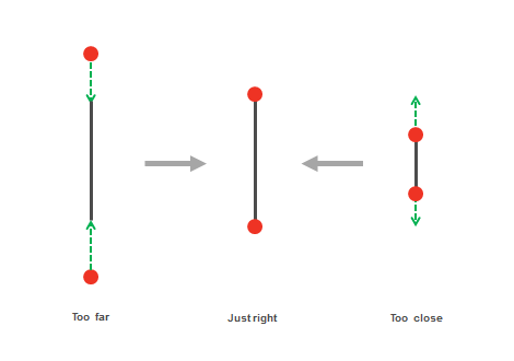
Normally, calculating constraint forces for a complex system can be quite strenuous. Luckily, applying constraints in a Verlet system is very straightforward due to the fact the particle's previous position is saved. When the particle moves past the maximum length of the spring, we simply move it back to a position within the constrained length without calculating the resulting velocity.

// Vector from neighbor position to self position
Vector it2me = p1.pos - p1.pos;
// Current length of spring
float length = it2me.magnitude();
// Check if length is within min/max limit
if (length < MIN || length > MAX) {
    // Apply constraint
    if (length < MIN) length = MIN;
    if (length > MAX) length = MAX;
    // Scale vector to to constraint length
    it2me = it2me.normalize() * length;
    // Find midpoint between particle and its neighbor
    Vector midpt = (p1.pos + p2.pos) / 2.0;
    // Apply constraint to particle and its neighbor by
    // moving them towards or away from each other
    p1.pos = midpt + (it2me / 2.0);
    p2.pos = midpt - (it2me / 2.0);
}
            

The above code processes semi-rigid constraint for spring connections. For a rigid constraint, instead of keeping the distance between two particles to a minimum or maximum length, just set it to a single length.

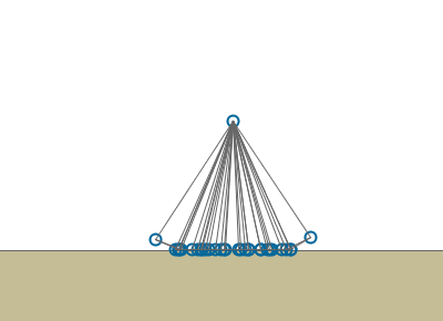
Even with constraints, a system can become unstable and collapse. One reason may be that as you satisfy constraints for one part of the system, another part becomes unstable, which then causes yet another part to become unstable, creating a ripple effect throughout the system. Also, since our spring constraint only measures absolute distance between particles, if a particle moves too far to the other side of its neighbor, the constraint will keep it on the "wrong" side. As a result, instead of staying in the shape of a ball, the particle system collapses in on itself.

One quick and dirty way to fix this problem is to create some more spring constraints around the blob. A better approach is to use a method called relaxation, where the constraint function is run multiple times so that it eventually converge to a stable solution. Of course, the greater the number of iterations, the more your simulation's performance suffers, so you will need to play around with the system to find the optimal number of iterations.

Keep in mind that you should calculate forces acting on all particles first, then move all of them, and finally handle all constraints. When a particle moves, the extra force it distributes to its neighbor will be different from the original force its neighbor is supposed to take in. The problem is amplified when you apply the constraint before movig on to the next particle, causing a large ripple effect that will destabilize the system, which will wobble around in the absence of external forces.

One strange behavior worth mentioning is that even with a very tight (or rigid) constraint, a system would deform if it is pushed up against the edge of the world. Not so rigid! The cause was the order in which constraints and collisions were processed: A part of the collision function checks if a particle is outside the world boundary, if it is, the particle is projected back into the world. The fact that this is done after satisfying constraints meant particle position can be still be outside of their constraint. The lesson? Make sure the constraints are properly applied!

// Calculate them separately!
for (int i = 0; i < num_of_particles; i++) {
    AccumulateForces(particle[i]);
}   
for (int i = 0; i < num_of_particles; i++) {
    VerletIntegration(particle[i]);
}
// Relaxation loop
for (int j = 0; j < relax_iteration; j++) {
    for (int i = 0; i < num_of_constraints; i++) {
        SatisfyConstraints(constraints[i]);
    }
}
            

+ Resources

• Cowboy Programming - Blob Physics
• Thomas Jakobsen - Advanced Character Physics
• BlueThen - Curtain and How To Build a Fabric Simulator
• Andrew Witkin - An Introduction to Physically Based Modeling: Constrained Dynamics

# Physically Based

A very simple collision detection method is used here: If a particle moves out of the world bounding box, we use the direction it was moving towards as well as its force to calculate a new direction parallel to the border (adjusted by a friction coefficient).

Within a Verlet system, the previous position is readily available to make all of this extremely simple. Sometimes the particle may get stuck outside of the bounding box, in which case the particle is simply moved back just inside the bounding box border.

With the collision system in place, we now move our attention to the blob itself. A blob is made up of a system of spring-connected particles, the appearance and behavior of the blob depends heavily on the internal structure of the springs and particles. Within a system, differences in spring length and elasticity, as well as particle size, can result in vastly difference blobs. Different constructions have their own strengths and weaknesses. Getting a specific blob system to behave just right often takes a lot of trial and error. Below are some of the more commonly used builds that serve as a solid starting point.

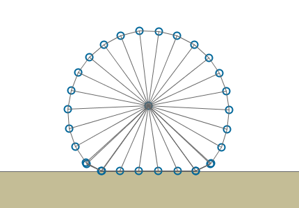
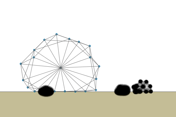
A single-skinned blob: A circle of particles were each particle is joined to its left and right neighbors, as well as to a particle in the center. This is a straightforward structure to implement and allows reasonable performance. However, the simplicity of its structure also gives rise to several problems: The single-layered skin can easily get caught and fold over each other. Depending on the stiffness of the spring, the entire blob can sometimes collapse in on itself.

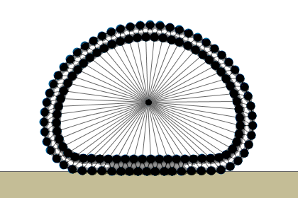
A double-skinned blob: Discussed in-depth in this article, this is created with two interconnected layers of particles with one particle in the center. It is more stable than the single-skinned blob and can produce very realistic movements. Due to its more complex structure, more time is needed to tweak the spring constraints to get things to behave "just right." Also, performance takes a hit due to the added complexity, and a large blob can slow the simulation down to a crawl.

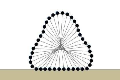
An interconnected blob: Unlike the skinned blobs, it has no center point mass. To make up for the lack of an internal support, each particle is connected to its neighbors as well as its opposing particle (the game Gish uses a similar method). The additional springs result in a stable structure that is unlikely to collapse on itself.

+ Resources

• GameDev.net - A Verlet based approach for 2D game physics
• N Tutorial A - Collision Detection and Response
• Cowboy Programming - Blob Physics
• Wolfire Games Blog - Early Gish hacking

# Rendering

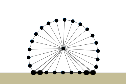
With a solid mass-spring structure in hand, we use metaballs to render the actual blob. In computer graphics, metaballs are organic-looking circular objects that blend into closeby metaballs to form a gooey, blobby-looking entity.

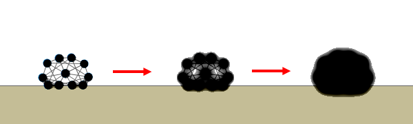
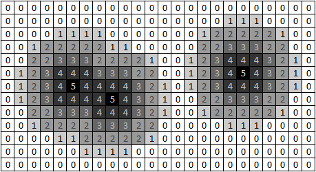
Mathematically, metaballs are defined by a function that calculates a value for a given pixel based on its distance relative to all other metaballs on the screen. Pixels in between two metaballs is "colored" by both, thus creating the effect where the two metaballs are "melting" into each other. The metaball equation is as follows:

P(x, y) = R / sqrt((x - x₀)² + (y-y₀)²)

Where R is the metaball radius, (x, y) and (x₀, y₀) are coordinates of the current pixel and the metaball, and P(x, y) is the resulting color. Just by looking at the equation, we see that if the pixel is located at the center of the metaball, then x = x₀ and y = y₀, the denominator goes to 0, and P(x, y) goes to infinity (or, in our case, the pixel ends up being black). As we move further away, the denominator becomes smaller, giving us lighter pixel colors.

The basic algorithm to render a blob is then:

1. Iterate through every on-screen pixel
2. For each pixel, iterate through every particle
3. Use the metaball equation to calculate the pixel's color

Only one problem left... notice there is a square root in our metaball function. Square roots tend to be computationally expensive, especially when the operation is done for every single pixel! There are many ways to optimize the algorithm, for our system we will use two simple tricks to achieve big speed boosts.

First, notices how only a small portion of the pixels on-screen are needed to render the metaballs. Instead of iterating through every single pixel, bounding boxes are put around each blob. During rendering, only pixels within those bounding boxes are computed. The second optimization is to eliminate the square root entirely. By doing so, we need to change the numerator part of the equation to compensate for the larger denominator.

Combining the above two optimizations, the rendering algorithm then becomes:

1. Calculate metaball bounding boxes and cache the pixel coordinates
2. Iterate through every cached pixel
3. For each pixel, iterate through every particle
4. Calculate the pixel's color using the function: P(x, y) = (R * metaball_size) / [(x - x₀)² + (y-y₀)²]

// Iterate through each cached pixel
for (each pixel in cache) {
    float sum = 0.0;
    // Iterate through all particles
    for (each p in particles) {
        // Calculate pixel value using modified metaball equation
        sum += p.radius*metaball_size / (sq(p.pos.x - x) + sq(p.pos.y - y));
    }
    // If resulting sum is greater than a pre-defined threshold, render the pixel as metaball
    if (sum > metaball_band) {
        pixels[index] = color(sum);
    }
}
            

+ Resources

• GameDev.net - Exploring Metaballs and Isosurfaces in 2D
• Ryan Geiss - Metaballs (also known as: Blobs)
• Hannu's Plaza - Metaball math
• Processing - Optimization metaball effect

# Results

This is a simple blob simulation that incorporates some of the popular techniques found in games and physics engines. For more in-depth discussions of topics such as Verlet Integration and Metaballs, follow the reference links found at the end of in each section. There are many more ways to improve the realism and performance of the simulation, the materials found here should serve as a good starting point for aspiring blob adventurers!